Dynamic Defect Detection
by Neil Coleman, President/CEO Signalysis,
Inc. and Robert Coleman, Senior Applications Specialist for
Signalysis, Inc.
(Note: Due to formatting limitations
in HTML, it may be difficult to read formulas properly.)
Wide-ranging measurement methods are applied on
the assembly lines of production plants across the country.
The ever rising bar of quality demands rejection of defective
products at an assurance level not imagined in years past. The
future of defect detection is perhaps in the identification
of assembly line units that are not yet defective, but would
otherwise be expected to fail prematurely in the hands of the
consumer.
A production test activity once dominated by mechanically operated
micrometers now is characterized by computer controlled measurement
devices and data acquisition and analysis systems. Yet, many
production plants have not taken advantage of newly developed
methods of dynamic measurement and signal processing.
This article suggests dynamic testing as a means of detecting
not only on-the-line defects, but also the potential for premature
failure after delivery to the customer.
The Dynamic Measurement Concept
It has been found that a large variety of products possess
intrinsic dynamic characteristics that provide a signature of
the state of their health. Sometimes these characteristics are
chemical, optical, electrical, magnetic or mechanical in nature.
Regardless, there is much commonality in the basic measurement
and analysis process applied in assessing the state of product
health.
The key feature of the dynamic process is the integration of
fast, continuous response measurement devices, high-speed data
acquisition, advanced time and frequency domain signal processing,
data analysis and production line disposition and control. Further,
integration on the analysis side should merge statistical analysis
methods with techniques of time and frequency domain finger
printing.
The present article will focus on the use of mechanical vibration
characteristics for rating product health. However, methods
described here apply to measured parameters associated with
other kinds of product characteristics.
Single Degree Of Freedom Vibration Theory
Most products, from small to large… from components, computers,
TV sets, appliances, motors and equipment to vehicles, aircraft,
bridges and buildings, are rich in vibration characteristics
which can indicate their state of health. The reason is that,
in a mechanical dynamical sense, these products are all composed
of quite a large number of masses, springs and dampers. And
every combination of a mass, spring and damper has associated
with it a resonance frequency and a mathematical characteristic
we call the SDOF FRF (Single-Degree-Of-Freedom Frequency Response
Function). The combination of many masses, springs and dampers
within a product results in many resonance frequencies along
with the superposition of their FRF's. The FRF resulting from
this superposition manifests a myriad of markers useful for
assessing product integrity.
The FRF is fundamental to the understanding of the richness
of intrinsic vibration characteristics of a product. The subject
of vibration measurements has been presented in three recent
issues of the Sensors magazine (February, March and April) and
is recommended reading for the understanding of our present
application. The FRF is a mathematical function derived using
measurements of an applied dynamic force along with the vibratory
response motion. The response motion could be displacement,
velocity or acceleration.
The FRF concept can be understood in association with the simple
mass, spring and damper diagrammed in Figure 1. A vibratory
force, f(t), is applied to the mass, inducing response vibration
displacement, X(t). The applied force is typically a random
time function having a continuous spectrum over the frequency
range of interest. The FRF results from the solution of the
differential equation of motion for the SDOF system.
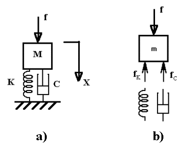 |
| Figure 1.
A vibratory force is applied to a simple mass, spring and
damper system, a). The differential equation of motion is
developed from the free-body diagram , b). This equation
describes the vibration displacement response of the system.
|
The differential equation of motion for the SDOF
system is obtained by setting the sum of forces acting on the
mass equal to the product of mass times acceleration (Newton's
Second Law):
 (equation1)
where f(t) represents the time dependent force
(LB), x is the time dependent displacement (inch), m is the
system mass, k is the spring stiffness (LB/inch) and c is the
viscous damping (LB/in/sec).
The FRF is a frequency domain function, and we
derive it by first taking the Fourier Transform of equation
(1). One of the benefits of transforming the time dependent
differential equation is that a fairly easy algebraic equation
results, owing to the simple relationship between displacement,
velocity and acceleration in the frequency domain. These relationships
lead to an equation that includes only the displacement and
force as functions of frequency. Letting F( )
represent the Fourier Transform of force and X()
represent the transform of displacement,
)
represent the Fourier Transform of force and X()
represent the transform of displacement,
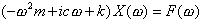 (equation2)
The circular frequency, ,
is used here (radians/sec). The damping term is imaginary, due
to the 90-degree phase shift of velocity with respect to displacement
for sinusoidal motion. Now, the FRF is obtained by solving for
the ratio of the displacement Fourier Transform to the force
Fourier Transform. The FRF is usually indicated by the notation,
h().
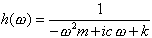 (equation3)
(3) After rationalizing the denominator and defining
some key parameters in a more popular form, equation (3) is
written as
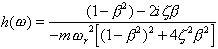 (equation4)
This form of the FRF allows one to recognize the
real and imaginary parts separately. The new parameters introduced
in equation (4) are the frequency ratio,  =
/
r, and the damping factor,
=
/
r, and the damping factor,  .
The understanding of these parameters becomes clearer when considering
two different ways of inducing vibration on the SDOF system.
Figure 2 illustrates the vibration behavior under forced sinusoidal
vibration with a continuously increasing frequency compared
to vibration resulting from a sudden impact. The upper diagram
of Figure 4 depicts a process in which a computer controlled
electrodynamic shaker impresses a vibration force that slowly
sweeps up from a low frequency to a high frequency. The mass
and spring respond with amplified vibration as the shaker sweeps
into that special frequency range of system resonance. The level
of vibration response when forced at the resonance frequency,
r, depends on the amount of damping as quantified by
the damping constant, C. The damping factor, ,
is the ratio of actual damping, C, to the damping value known
as critical damping, Cc. A system with
equal to or greater than 1.0 will not vibrate freely. Typical
product values of
range from .01 to .05, except for products specifically designed
with high damping,
> 0.1, to inhibit vibration.
.
The understanding of these parameters becomes clearer when considering
two different ways of inducing vibration on the SDOF system.
Figure 2 illustrates the vibration behavior under forced sinusoidal
vibration with a continuously increasing frequency compared
to vibration resulting from a sudden impact. The upper diagram
of Figure 4 depicts a process in which a computer controlled
electrodynamic shaker impresses a vibration force that slowly
sweeps up from a low frequency to a high frequency. The mass
and spring respond with amplified vibration as the shaker sweeps
into that special frequency range of system resonance. The level
of vibration response when forced at the resonance frequency,
r, depends on the amount of damping as quantified by
the damping constant, C. The damping factor, ,
is the ratio of actual damping, C, to the damping value known
as critical damping, Cc. A system with
equal to or greater than 1.0 will not vibrate freely. Typical
product values of
range from .01 to .05, except for products specifically designed
with high damping,
> 0.1, to inhibit vibration.
The lower diagram of Figure 2 reflects that same
resonant property of the spring-mass system. The mass and spring
are shocked into vibration at the system resonance frequency.
The vibration dies away with time at a decay rate dependent
on the damping constant, C.
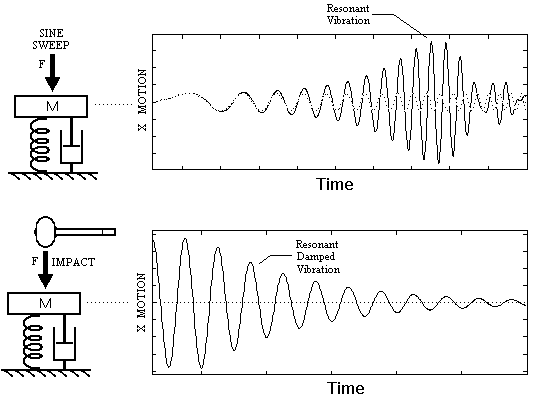 |
| Figure 2. Vibration response
of a SDOF system to two different excitation processes.
The upper diagram shows response to an applied sine sweep
forcing function. The lower diagram shows response to a
hammer impact force. |
Actually, either of the two displacement-time
functions plotted in Figure 2 could be derived from the differential
equation (1). Just enter either the sine sweep forcing function
or the hammer impact force for f(t) in equation (1) and solve
for the displacement response. But, an efficient use of the
data from either of the vibration processes would be to Fourier
Transform force and displacement measurements and compute the
FRF. This result is sketched in Figure 3.
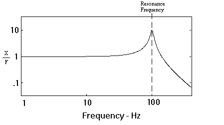 |
| Figure 3. The FRF
(Frequency Response Function) plot for the SDOF of Figure
1. The FRF could be computed from the Fourier Transform
ratio of X()/F()
using data from either of the Figure 2 vibration processes.
The FRF peaks at the system resonance frequency,
r. |
The FRF of Figure 3 directly reflects the sine
sweep process. The system response is fairly constant throughout
the low frequency range and rises to a peak at the resonance
frequency, r.
The resonance frequency can be shown to depend on the system
mass and stiffness:
 (equation5)
Multiple Degree Of Freedom Systems
There is a reason for this extensive excursion
into SDOF vibration theory. It is because the most complicated
structure, having a large number of masses and springs and resonance
frequencies can be understood as a superposition of simple SDOF
systems. Such a complicated system is thought of as a MDOF system
(Multiple-Degree-Of- Freedom system) having many modes of vibration.
The resulting complicated FRF can be understood as a mathematical
summation of SDOF FRF's, each having a resonance frequency,
damping factor, modal mass, modal stiffness and modal damping
ratio.
A complicated structure need not have distinct
lumped masses and springs to be analyzed as a MDOF system. Product
structural elements such as beams and panels represent MDOF
components, given their many different modes of bending. Figure
4 summarizes the way in which products may be visualized as
a superposition of SDOF modal components, even though lumped
masses and springs are not involved. A cantelever beam serves
as the example, exhibiting unique deformation patterns called
mode shapes. The beam can be made to vibrate freely in any of
the individual mode shapes, and again, associated with each
mode shape is a resonance frequency, modal mass, modal stiffness,
modal damping and a modal FRF.
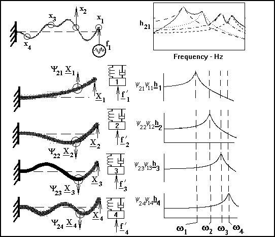 |
| Figure 4. A cantelever beam exhibits
distinct vibration deformation patterns. Each deformation
pattern, called a mode shape, behaves like a SDOF component.
The measured FRF (upper right corner), X2/F1,
is understood as a superposition of the SDOF FRF's. |
A useful thing to know about vibrating structures
is that they can only vibrate using these unique mode shapes.
Any arbitrary deformation produced in a vibration process (such
as the upper left corner example of Figure 4 can only occur
if it is comprised of the superposition of the natural mode
shapes. This understanding, along with knowledge of the way
in which the presence of specific vibrating mode shapes are
manifest in measured data, arms one with valuable tools for
establishing strategies for product defect detection.
Mode Shape Mathematics
A powerful mathematical concept presents mode
shapes as a vehicle for transforming vector components like
displacement, velocity, acceleration and force from their natural
physical coordinate system to an abstract modal coordinate system.
A matrix of mode coefficients,  jr,
represents all of the mode shapes of interest of a structure.
The mode coefficient index, j, locates a numbered position on
the structure (a mathematical degree of freedom) and the index,
r, indicates the mode shape number. Modes are numbered in accordance
with increasing resonance frequencies. The vector component
coordinate transformation from abstract modal coordinates, X,
to physical coordinates, X, is
jr,
represents all of the mode shapes of interest of a structure.
The mode coefficient index, j, locates a numbered position on
the structure (a mathematical degree of freedom) and the index,
r, indicates the mode shape number. Modes are numbered in accordance
with increasing resonance frequencies. The vector component
coordinate transformation from abstract modal coordinates, X,
to physical coordinates, X, is
{ X } = []{
X } (equation6)
Each column in the [
] matrix is a list of the mode coefficients describing a mode
shape. Figure 4 shows the modal displacements, X1,
X2, X3
and X4, defined at the end of the
cantelever beam for each mode shape. As an example of the coordinate
transformation, we see that the physical displacement at position
number two, X2 (see Figure 2 upper left
corner), is equal to the sum of the modal displacements weighted
by the corresponding mode coefficients.
Now, any system having mass, stiffness and damping
distributed throughout can be represented with matrices. Using
such matrices a set of differential equations can be written
for the Figure 2 cantelever beam, for example. The frequency
domain form is
 (equation7)
(7) Displacements and forces at the numbered positions
on the structure appear as elements in column matrices. The
mass, damping and stiffness matrix terms are usually combined
into a single dynamical matrix, [ D ]:
[ D ]{ X } = { F } (equation8)
A complete matrix, [ H ], of FRF's would be the
inverse of the dynamical matrix. Thus, we have the relationship,
{ X } = [ H ]{ F } (equation9)
Individual elements of the [ H ] matrix are designated
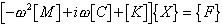
with the notation, hjk(),
where the j index refers to the row (location of response measurement)
and the k index refers to the column (location of force). A
column of the [ H ] matrix is obtained experimentally by applying
a single force at a numbered point, k, on the structure while
measuring the response motion at all n points on the structure,
j = 1,2,3…n. The [ H ] matrix completely describes a structure
dynamically. A one-time measurement of the [ H ] matrix defines
the structure for all time… until a defect begins to develop.
Then subtle changes crop up all over the [ H ] matrix. From
linear algebra we have the transformation from the [ H
] matrix in modal coordinates to the physical [ H ] matrix.
[ H ] = [
][ H ][ ]T2
(equation10)
This provides the understanding of a measured
FRF, hjk(),
as the superposition of modal FRF's. Equation (10) may be expanded
for any element of the [ H ] matrix (selecting out a row and
column) to obtain the result,
 (equation11)
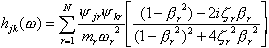
Equation (11) is illustrated graphically in the
upper right corner of Figure 2. The solid FRF curve, h21,
is shown as an algebraic summation of the weighted modal FRF's
adjacent to each of the beam mode shapes in the figure. The
resonance frequency of each mode of vibration depends on the
effective modal mass and effective modal stiffness associated
with each SDOF mode shape. The formula for modal resonances
is the same as equation (5):
 (equation12)
The modal damping fraction, r,
also depends on modal mass and modal stiffness as well as the
modal damping constant, cr. This is because
the critical damping value is a function of modal mass and modal
stiffness.
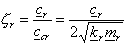 (equation13)
Another useful FRF parameter is the phase angle,
indicated by the real and imaginary parts of equation (11).
The phase angle function of frequency,  jk(),
associated with FRF hjk()
is
jk(),
associated with FRF hjk()
is
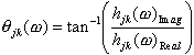 (equation14)
The vibration theory seems overwhelming at times.
Nevertheless, the multiplicity of modal parameters within a
single FRF can now be appreciated as providing such a rich source
of indicators of product health.
Potential Failure Detection
There is a particularly attractive feature of
dynamic defect detection using vibration measurements. It is
the possibility of adjusting rejection criteria for identification
of units having statistically significant potential for failure.
Mode shape definition, resonance frequency and
the modal damping factor are very sensitive to the mechanical
condition of a product. These parameters are so sensitive to
the state of a product that is not possible to manufacture two
units with precisely identical FRF's. Slight differences between
one unit and another will manifest as deviations between their
FRF's.
For example, a slightly loosened fastener can
affect those mode shapes having large mode coefficients in the
vicinity of the fastener. Notice in the FRF equation (11) the
effect of mode coefficients on the measured FRF. The loosened
fastener will also effect modal stiffness in those modes, which,
by equation (12) changes the resonance frequencies. Deviations
in mode coefficients and resonance frequencies show up as shifts
in FRF amplitude, locations of peaks and phase angle. The damping
factor, , may be
effected as a result of increased friction in loose joints.
This shows up in the FRF as a broadening of peaks as
increases. Figure 5 overlays two FRF's, differing as a result
of a slight change in just two of the structure modes. Two mode
coefficients have been altered along with a slight shift in
the two resonance frequencies and damping factors.
While an exact theory underlying the relevance
of vibration testing to failure potential is not fully developed,
the concept is based on fatigue theory. It has been suggested
that the fatigue life of certain components can be correlated
with their damping factor and resonance frequency. This would
mean that the future operating life of some components could
be estimated by measuring these modal parameters. On this basis
limits could be established for rejecting units not expected
to perform over a normal life span for the product.
Generally speaking, there are two broad defect
detection strategies: 1) Theory-Based and 2) Phenomenological.
The theory-based strategy attacks the problem with full knowledge
of the product dynamical characteristics. The phenomenological
strategy employs the same measurement and signal processing
methods, but without knowledge of the system model. Both strategies
provide the possibility of detecting the potential for premature
failure.
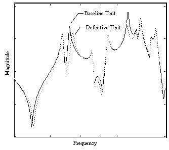 |
| Figure 5. Comparison of FRF's
for a baseline unit under test and a defective unit. Two
modes have been affected by the defect, resulting in shifts
in resonance frequencies, damping ratios and mode coefficients. |
Theory-Based Defect Detection Strategies
The theory-based strategy includes experimental
development of the global modal parameters, r,
mr, kr
and r
along with the physical and modal FRF matrices, [ H ] and [
H ], and the mode shape matrix, [
]. A standard process yielding this body of data is referred
to as a modal test. The development of laboratories for performing
modal tests is becoming more and more common in industry.
Also, Finite Element Modeling is often pressed
into service as part of the strategy. Experimental modeling
and analytical modeling provide a very effective approach when
the two technologies are properly coordinated. The two methods
are complimentary in many ways. Each has advantages and disadvantages
when compared to the other.
Having an understanding of the modal characteristics
of a product enables the development of multiple failure mode
strategies. The mechanisms associated with different failure
modes can be understood in relation to the various mode shapes
and resonance frequencies of a product.
The theory-based strategy lends itself to strategically
placed measurement devices (typically accelerometers or laser
vibrometers). A quick glance at the mode shapes for the cantelever
beam in Figure 4 indicates the end of the beam assures data
that will involve every mode of the structure. An accelerometer
positioned at a zero crossing for a particular mode shape will
fail to produce any information about the health of that mode.
The mode coefficient at that point would be zero and would remove
that mode from the modal FRF summation as seen in equation (11).
Assembly line vibration testing may involve an
active operating product or a passive product. An operating
electric motor provides its own vibration excitation. In this
case the theory-based strategy provides an understanding of
the modal forces generated by the motor. Having a modal model
enhances the development of a test strategy.
A major pitfall in the implementation of the vibration
defect detection method has to do with assembly line fixture
design. Without an understanding of the way the unit under test
is dynamically coupled to the fixture, the whole process could
fail. Some plants have been found rejecting good units based
on vibration measurements effected largely by fixture dynamics.
This problem is easily avoided with a theory-based strategy
in which all system characteristics, including fixture, are
understood up front.
The analytical approach to defect detection requires
special facilities and human resources. The technology is costly
to implement and maintain in-house. Companies often prefer to
rely on outside consultants to initiate the process and bring
the assembly line into a routine production operation. Once
the process is in place for a particular product, little specialization
is required as long as the product is not subject to redesign.
Phenomenological Strategy
This strategy takes advantage of the dynamic
characteristics of the product without really understanding
the behavior. Dynamic measurement levels may be established
across the frequency spectrum for an adequate statistical sample
of good units. Then, out-of- tolerance levels are established
as a basis for rejecting defective or potentially defective
units. Plants engaging this strategy usually go through an extended
period of tweaking failure criteria and limits before reaching
a stable pass-fail process.